Kevin Waters An Academic Portfolio
Projected Band Structure and DOS (Individual Atoms)
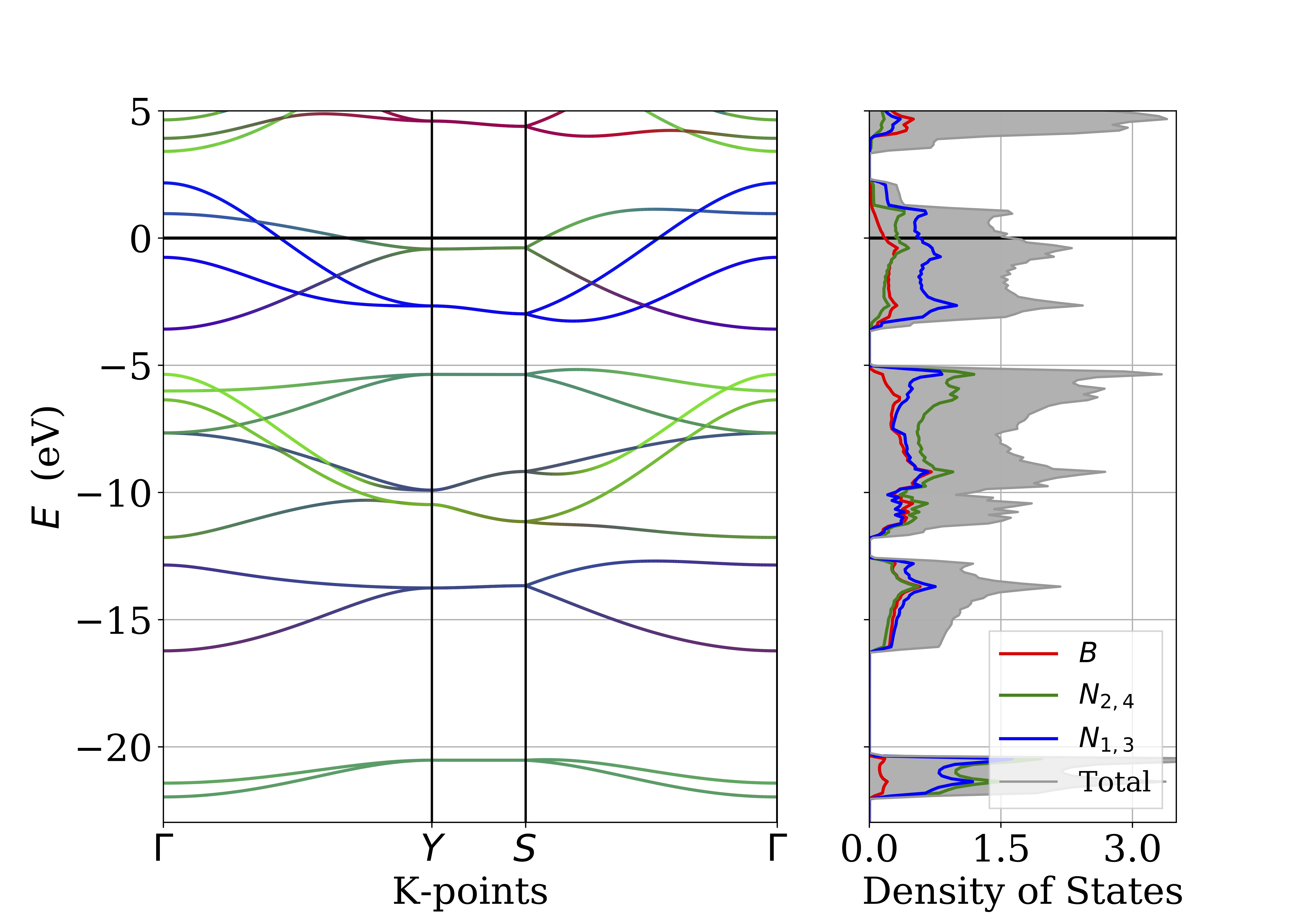
This is a continuation from the previous post on plotting the projected band structure and density of states. This will be as a standalone post, so there will be repeated elements in the code.
Due to the nature of plotting individual atoms, using the code requires more effort. In the current set up there are comments “### CUSTOM ATOM CHOICES” where code will need to undergo significant changes to be adapted to another system. It is currently set up to graph three sets of atoms that are based of a past project. The code could be made to be more modular and user friendly for the inputs.
Previous post notes
The program is based of the original posted by here. This is a code I still want to come back to and reorganize, but it is functional in its current state. It plots the orbital projected band structure and density of states for a VASP calculation. At the bottom of the page is a .zip file with the contents needed to give it a test run. Some manual inputs for kpoint spacing and labels (Can be fixed), found under the comment #labels.
Files Needed
1) Band structure vasprun.xml
2) Band structure KPOINTS
3) Band structure PROCAR
4) PDOS vasprun.xml
Code
from numpy import array as npa
import numpy as np
import math
import pymatgen
import sys

#Import VasprunClass
from pymatgen.io.vasp.outputs import Procar, Vasprun
from pymatgen import Structure
from pymatgen.electronic_structure.core import Spin, Orbital

import matplotlib.pyplot as plt
from matplotlib.collections import LineCollection
from matplotlib.gridspec import GridSpec

def rgbline(ax, k, e, red, green, blue, KPOINTS, alpha=1.):
    #creation of segments based on
    #http://nbviewer.ipython.org/urls/raw.github.com/dpsanders/matplotlib-examples/master/colorline.ipynb
    pts = np.array([KPOINTS, e]).T.reshape(-1, 1, 2)
    seg = np.concatenate([pts[:-1], pts[1:]], axis=1)
    nseg = len(KPOINTS) -1
    r = [0.5*(red[i]+red[i+1]) for i in range(nseg)]
    g = [0.5*(green[i]+green[i+1]) for i in range(nseg)]
    b = [0.5*(blue[i]+blue[i+1]) for i in range(nseg)]
    a = np.ones(nseg, np.float)*alpha
    lc = LineCollection(seg, colors=zip(r,g,b,a), linewidth = 2)
    ax.add_collection(lc)


if __name__ == "__main__":

    bands_K = Vasprun("./BAND/vasprun.xml")
    structure = Structure.from_file("./BAND/POSCAR")
    bands = Vasprun("./BAND/vasprun.xml").get_band_structure("./BAND/KPOINTS", line_mode = True)

    # projected bands
    data = Procar("./BAND/PROCAR").data
    # density of states
    dosrun = Vasprun("./PDOS/vasprun.xml")

    # labels (MANUAL INPUT NEEDED CURRENTLY HERE)
    labels=[u"$\\Gamma$", u"$Y$", u"$S$", u"$\\Gamma$"]
    # Number of points between kpoints, found in the KPOINTS file
    step = 150

    # general options for plot
    font = {'family': 'serif', 'size': 24}
    plt.rc('font', **font)

    # set up 2 graph with aspec ratio 2/1
    # plot 1: bands diagram
    # plot 2: Density of States
    gs = GridSpec(1, 2, width_ratios=[2,1])
    fig = plt.figure(figsize=(11.69, 8.27))
#    fig.suptitle("BN\textsubscript{2} Monolayer")
    ax1 = plt.subplot(gs[0])
    ax2 = plt.subplot(gs[1]) #, sharey=ax1)

    # set ylim for the plot
    # ---------------------
    emin = 1e100
    emax = -1e100

    bands.efermi = dosrun.efermi

    for spin in bands.bands.keys():
        for b in range(bands.nb_bands):
            emin = min(emin, min(bands.bands[spin][b]))
            emax = max(emax, max(bands.bands[spin][b]))

    emin -= bands.efermi + 1
    emax -= bands.efermi - 1
#    emin = -20
    emax = 5
    ax1.set_ylim(emin, emax)
    ax2.set_ylim(emin, emax)


    contrib = np.zeros((bands.nb_bands, len(bands.kpoints), 3))
    # sum up atomic contributions and normalize contributions
    for b in range(bands.nb_bands):
        for k in range(len(bands.kpoints)):
            nitrogen = 0
            nitrogen_sp = 0
            boron = 0
            for i in range(len(bands.structure.species)):
                # Sum over all orbital types
                # 0:s 1:py 2:pz 3:px 4:dxy 5:dyz 6:dz2 7:dxz 8:dx2_y2
                for j in range(0,8,1):
                    ### CUSTOM ATOM CHOICES
                    if str(bands.structure.species[i]) == "B":
                        boron += data[Spin.up][k][b][i][j]**2
                    if str(bands.structure.species[i]) == "N":
                        # Select atoms 3 and 5
                        ### CUSTOM ATOM CHOICES
                        if i == 3 or i == 5:
                            nitrogen_sp += data[Spin.up][k][b][i][j]**2
                        # Select the rest (atoms 4 and 6)
                        ### CUSTOM ATOM CHOICES
                        else:
                            nitrogen += data[Spin.up][k][b][i][j]**2
            tot = boron + nitrogen + nitrogen_sp
            ### CUSTOM ATOM CHOICES (Sets to be normalized need to be changed)
            if tot != 0.0:
                contrib[b, k, 0] = boron / tot
                contrib[b, k, 1] = nitrogen / tot
                contrib[b, k, 2] = nitrogen_sp / tot

    reciprocal = bands.lattice_rec.matrix/(2*math.pi)

    KPOINTS = [0.0]
    DIST = 0.0
    # Create list with distances between Kpoints (Individual), corrects the spacing
    for k in range(len(bands.kpoints)-1 ):
        Dist = np.subtract(bands.kpoints[k+1].frac_coords,bands.kpoints[k].frac_coords)
        DIST += np.linalg.norm(np.dot(reciprocal,Dist))
        KPOINTS.append(DIST)
    # plot bands using rgb mapping
    for b in range(bands.nb_bands):
        rgbline(ax1,
                range(len(bands.kpoints)),
                [e - bands.efermi for e in bands.bands[Spin.up][b]],
                contrib[b,:,0],
                contrib[b,:,1],
                contrib[b,:,2],
                KPOINTS)

    # style
    ax1.set_xlabel("K-points")
    ax1.set_ylabel(r"$E$  (eV)")
    ax1.grid()

    # fermi level at 0
    ax1.hlines(y=0, xmin=0, xmax=len(bands.kpoints), color="k", lw=2)

    TICKS = [0.0]
    for i in range(step,len(KPOINTS)+step,step):
        ax1.vlines(KPOINTS[i-1], emin, emax, "k")
        TICKS.append(KPOINTS[i-1])
    ax1.set_xticks(TICKS)
    ax1.set_xticklabels(labels)

    ax1.set_xlim(0, KPOINTS[-1])

    # Density of states
    # -----------------

    ax2.set_yticklabels([])
    ax2.grid()
    ax2.set_xticks(np.arange(0, 3.5, 1.5))
    ax2.set_xlim(0,3.5)
    ax2.hlines(y=0, xmin=0, xmax=3.5, color="k", lw=2)
    ax2.set_xlabel("Density of States")

    # atom contribution
    B_DOS = np.zeros(len(dosrun.pdos[0][Orbital.s][Spin.up]))
    N_DOS = np.zeros(len(dosrun.pdos[0][Orbital.s][Spin.up]))
    N2_DOS = np.zeros(len(dosrun.pdos[0][Orbital.s][Spin.up]))

    for i in range(len(bands.structure.species)):
        print("Summing Densities of State")
        print(str(bands.structure.species[i]) + " (" + str(i + 1) + " of " + str(len(bands.structure.species)) + ")")
        ### CUSTOM ATOM CHOICES
        if str(bands.structure.species[i]) == "B":
            B_DOS += npa(dosrun.pdos[i][Orbital.s][Spin.up]) + \
                     npa(dosrun.pdos[i][Orbital.px][Spin.up]) + \
                     npa(dosrun.pdos[i][Orbital.py][Spin.up]) + \
                     npa(dosrun.pdos[i][Orbital.pz][Spin.up])
        ### CUSTOM ATOM CHOICES
        if str(bands.structure.species[i]) == "N":
            # Select atoms 3 and 5
            if i == 3 or i == 5:
                N2_DOS += npa(dosrun.pdos[i][Orbital.s][Spin.up]) + \
                         npa(dosrun.pdos[i][Orbital.px][Spin.up]) + \
                         npa(dosrun.pdos[i][Orbital.py][Spin.up]) + \
                         npa(dosrun.pdos[i][Orbital.pz][Spin.up])
            # Select atoms 4 and 6
            else:
                N_DOS += npa(dosrun.pdos[i][Orbital.s][Spin.up]) + \
                         npa(dosrun.pdos[i][Orbital.px][Spin.up]) + \
                         npa(dosrun.pdos[i][Orbital.py][Spin.up]) + \
                         npa(dosrun.pdos[i][Orbital.pz][Spin.up])
    # Plot Labels
    ax2.plot(B_DOS,dosrun.tdos.energies - dosrun.efermi, \
            "r-", label = "$B$", linewidth = 2)
    ax2.plot(N_DOS,dosrun.tdos.energies - dosrun.efermi, \
            "g-", label = "$N_{2,4}$", linewidth = 2)
    ax2.plot(N2_DOS,dosrun.tdos.energies - dosrun.efermi, \
            "b-", label = "$N_{1,3}$", linewidth = 2)
    ax2.fill_between(dosrun.tdos.densities[Spin.up],
        0,
        dosrun.tdos.energies - dosrun.efermi,
        color = (0.7, 0.7, 0.7),
        facecolor = (0.7, 0.7, 0.7))

    ax2.plot(dosrun.tdos.densities[Spin.up],
        dosrun.tdos.energies - dosrun.efermi,
        color = (0.6, 0.6, 0.6),
        label = "Total")
    ax2.legend(fancybox=False, shadow=False, prop={'size': 18},loc=4)

    # Plotting
    # -----------------
    plt.savefig(sys.argv[0].strip(".py") + ".pdf", format="pdf")
File Download
The files can be downloaded here.
Written on March 25th, 2018 by Kevin Waters